Lifted 1.4 Documentation

by Gary Bollenbach

23 January 2020

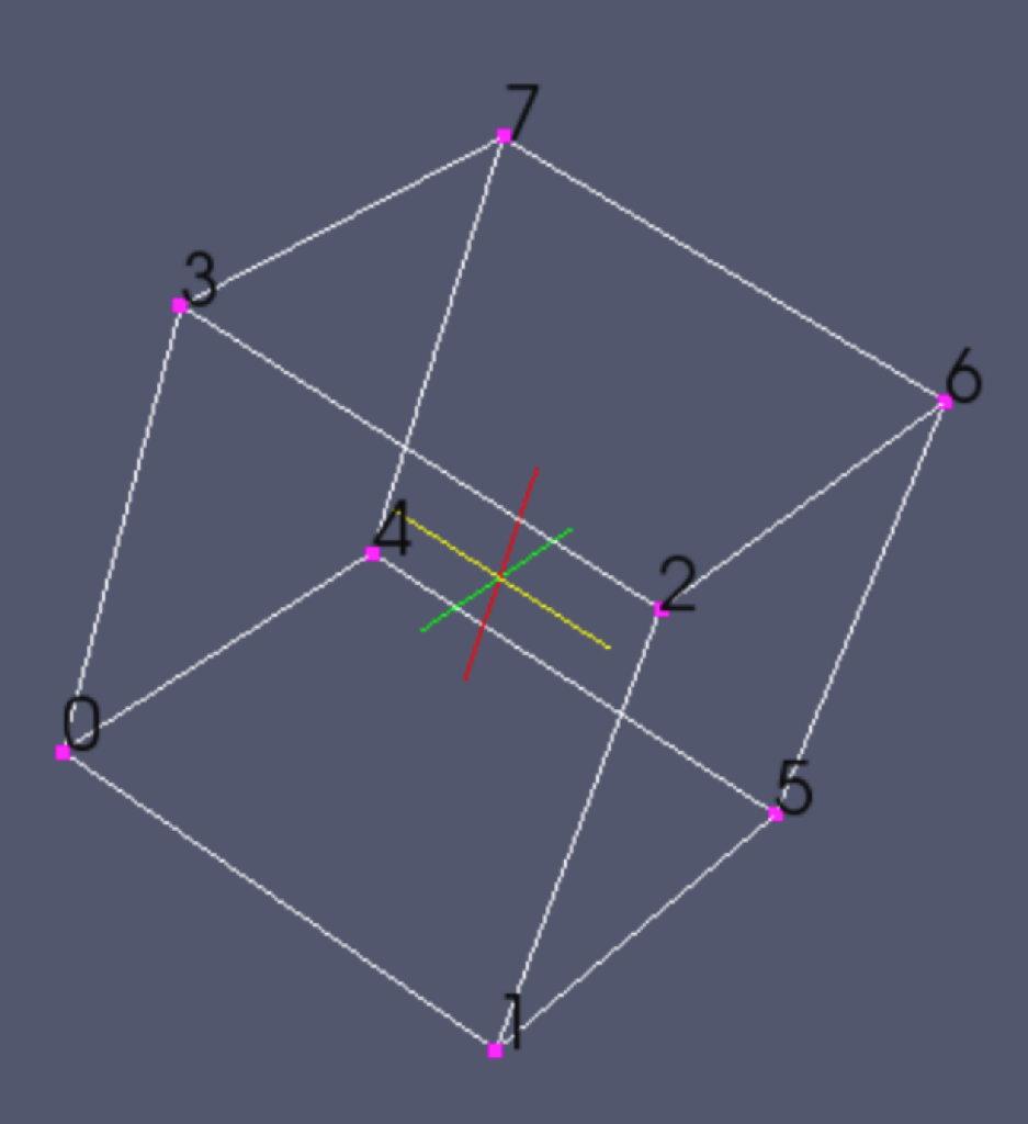
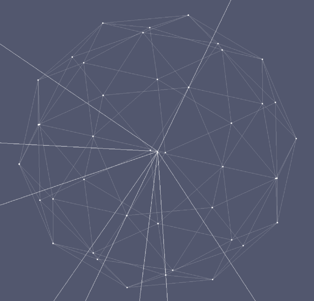
The pic to the right shows the way that Lifted works. The center node is shared by a number of elements, whose edges are seen here as radial lines. A polygon of points, here a twice subdivided ico-sphere consisting of 42 points, is created around the central node. A circuit is made in which a trial move of the central point places it sequentially at each of the ico points, and a quality attribute is evaluated there. The conditions represented by each position are analyzed and saved. Then, if the average quality of the entire group of elements improves when the point is located at the most favorable trial position, that position is retained, and another vertex point (usually the worst case) is considered.
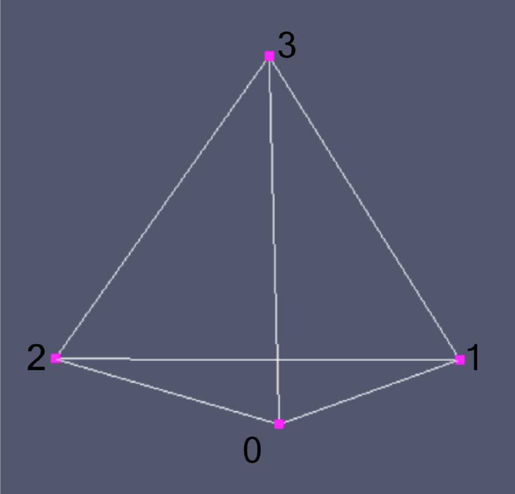
At right is an element with ordinary VTK node winding. Notice that (from the outside) the numbering can go clockwise or counter-clockwise, and that its outside direction reverses for the opposite face. This is not satisfactory for Verdict winding however. The Verdict requirement is for the first face listed to be wound clockwise. In other words, for the cube pictured, the line 8 0 1 2 3 4 5 6 7 would not be acceptable to Verdict, whereas the line 8 4 5 6 7 0 1 2 3 would be acceptable. For tetrahedra the Verdict requirement matches VTK. All VTK mesh which is opened by Lifted is rearranged, if necessary, to enforce Verdict requirements.
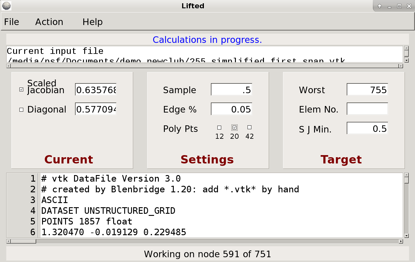
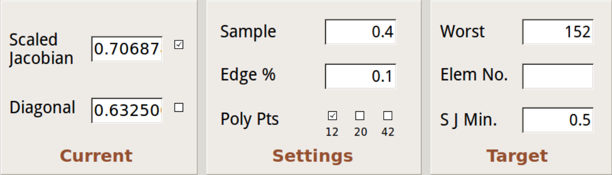
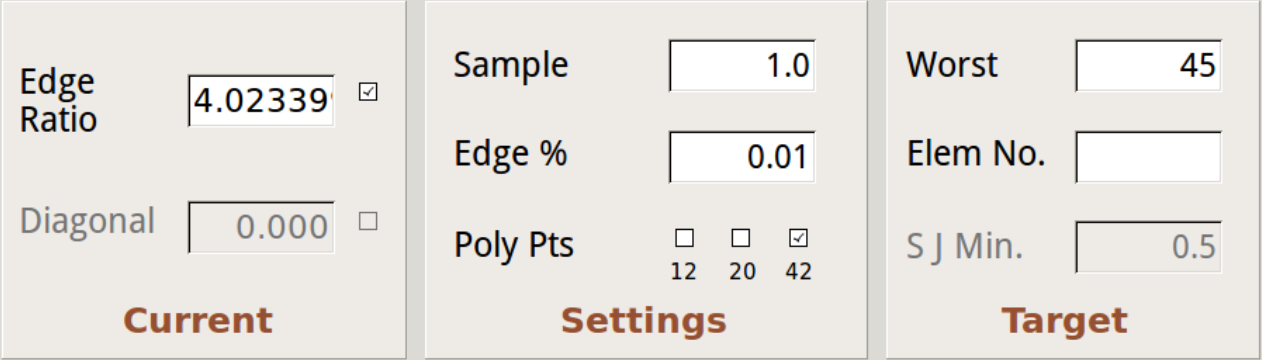
At right is the U/I. On the ‘Current’ panel are located the two Verdict quality standards used by Lifted, along with checkboxes to show which one controls the current calculations. The ‘Settings’ panel governs the geometrics of the trial positioning scheme. The ‘Target’ panel displays the least conforming element, a text box for single element treatment, and a quality guard factor. The Size button maintains the preferred U/I size. Normal termination of the Execute procedure is automatic, based on Sample size. However, a Stop option in the Action menu is available if early termination is desired. If saved immediately after selecting the Stop option, the saved file will show the quality levels displayed at the time of the stop.
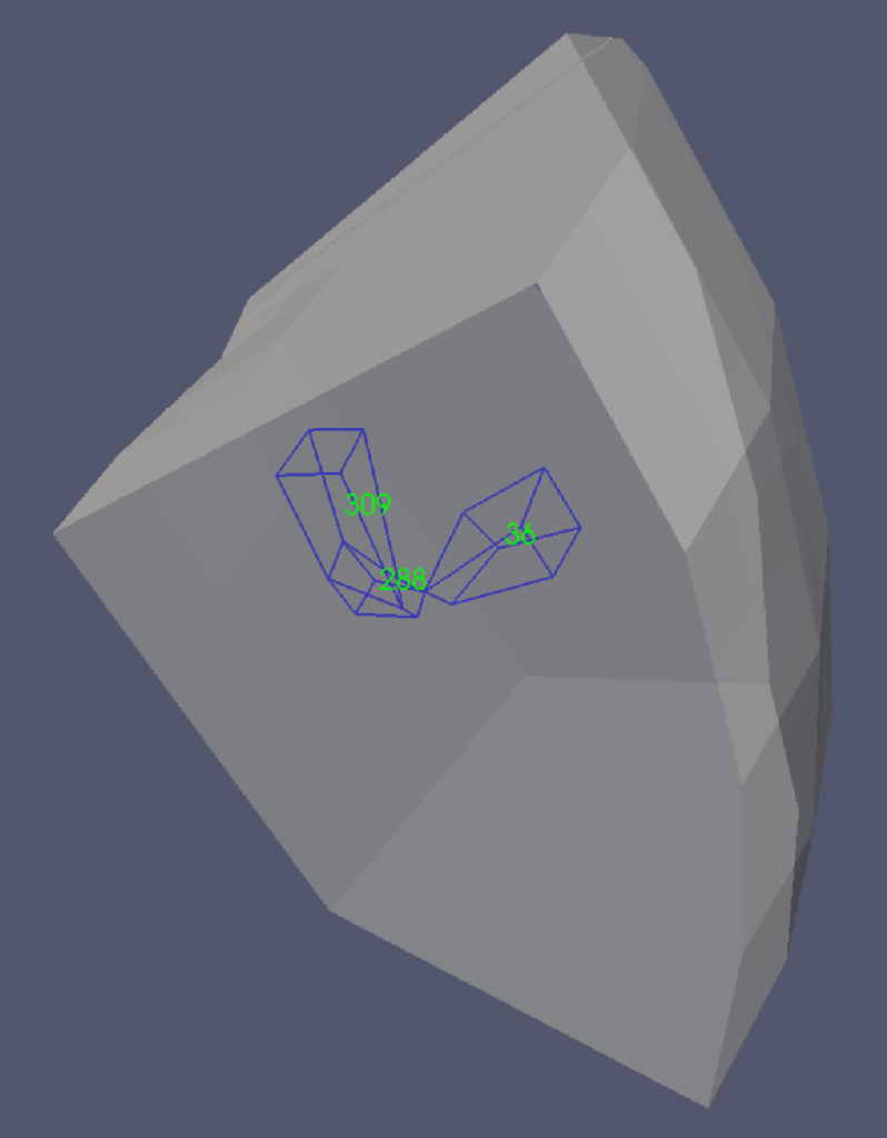
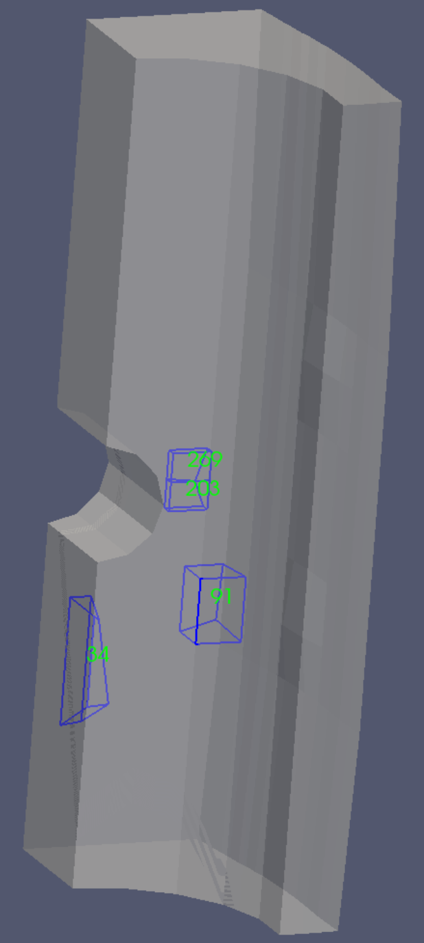
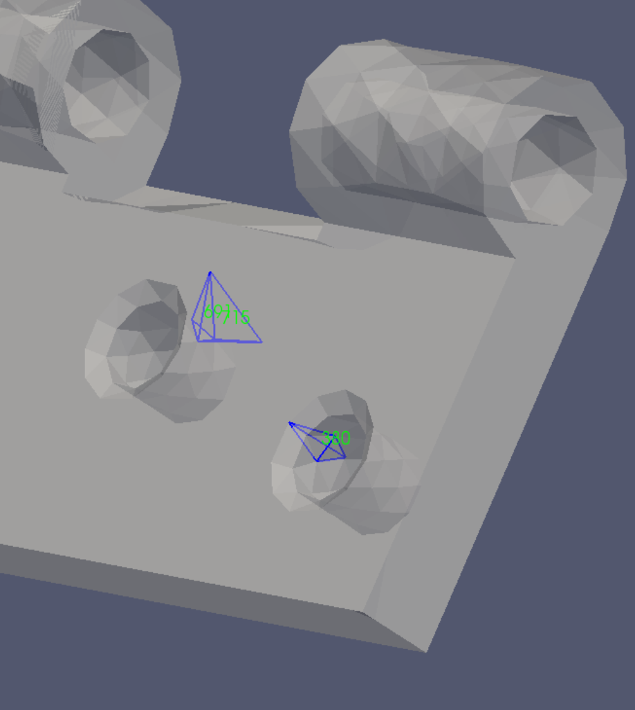
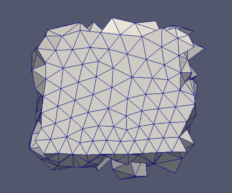
Demo 1 At right is shown the mesh for the first demo. It consists of a chunk of 312 hex elements with a partly rounded exterior. Three of its least regular elements are shown. Because none of the nodes for these elements reside on the mesh surface, Lifted may be able to accomplish a gain in quality. If, say, four nodes of a hex element were located on the surface, Lifted could still operate on the remaining internal nodes. We note that although Lifted can work on both hexahedral and tetrahedral mesh, the elements of the model must all be of the same type. Additionally, elements must be of 1st Order.
In regard to the U/I settings, the default Sample box factor of 1.0 means that the number of samples considered is 1.0 times the number of elements in the mesh. An excessive sample size does not hurt the results, but wastes time. If the Current panel has locked into a static display, but the node counter shown at the bottom of the U/I during calculations still has a considerable number remaining, the sample size is too big. If the ‘Current’ panel shows active change throughout the run, the sample size may be, but is not necessarily, too small. Generally, the larger the model, the smaller the sample size multiplying factor needs to be. The Edge % refers to the percent of the minimum edge length of the current node used to define the ‘radius’ of the test polyhedron. The Poly Pts checkboxes control the number of enclosed test points, making up either a 12-, 20-, or 42-point polyhedron.
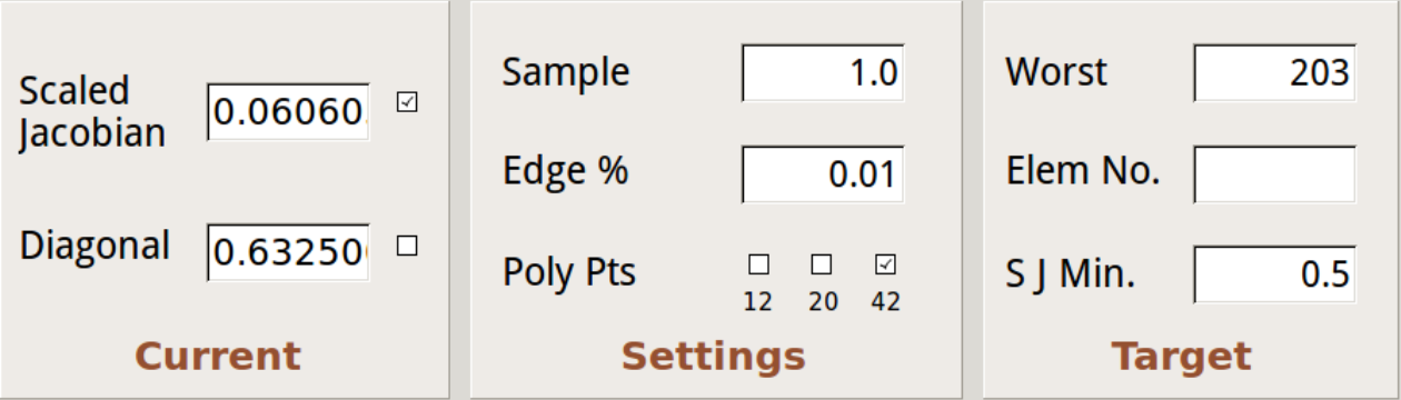
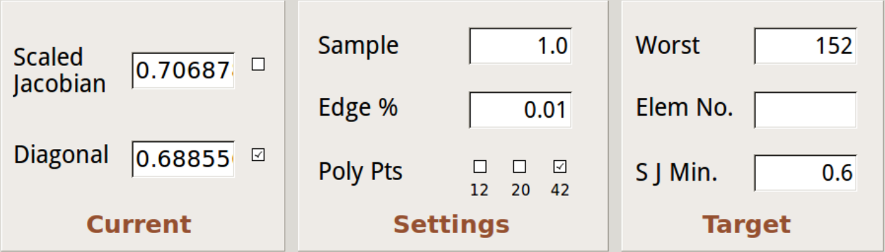
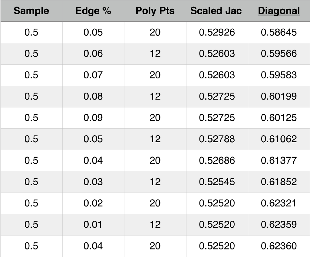
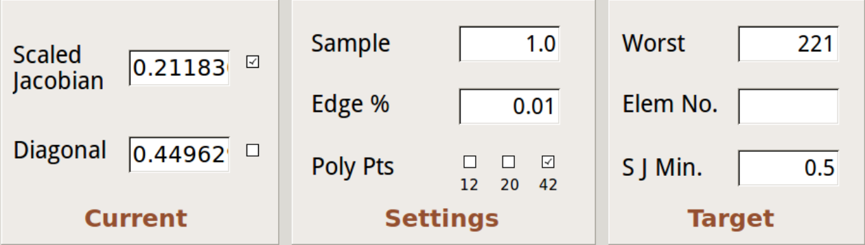
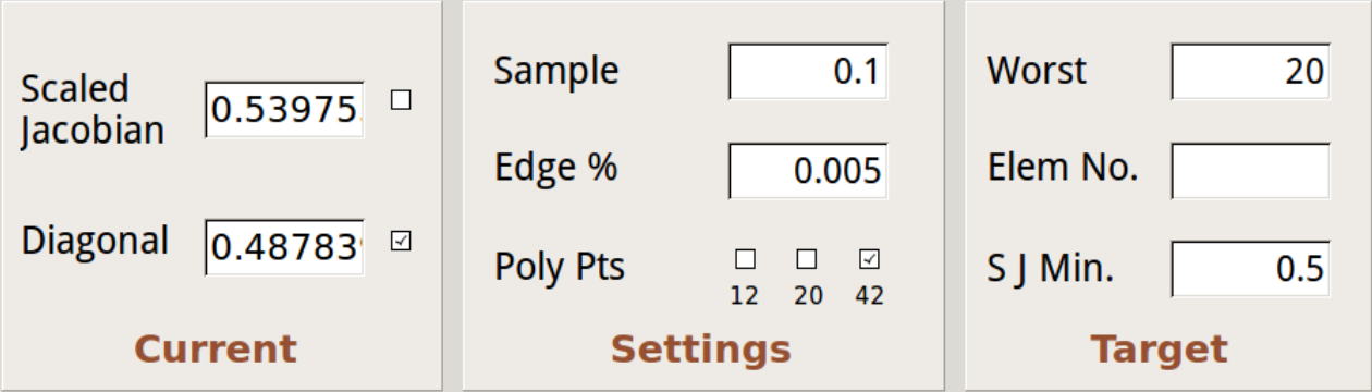
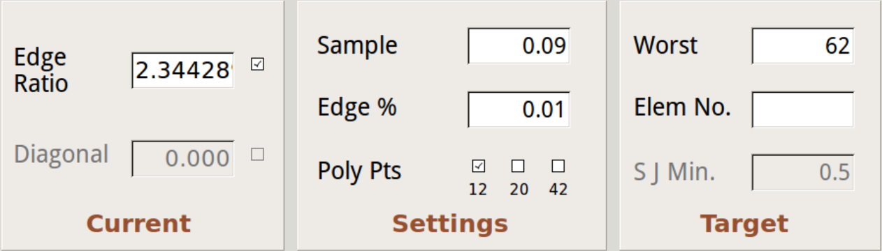
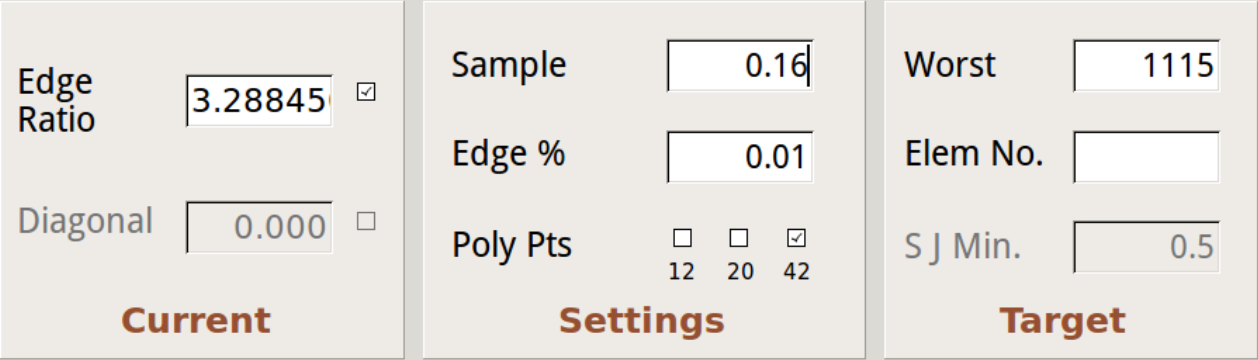
Reaching a satisfactory Scaled Jacobian value should suggest a save operation, to establish a reusable base for exploring possible Diagonal settings.		The Verdict standard for Scaled Jacobian of hexes is 0.5, and for Diagonal measure it is 0.65. The top table above shows the Scaled Jacobian and Diagonal scores of the demo file on opening. A single run with the Scaled Jacobian checkbox checked, and settings as shown in the second table, gives an improved value over the original. Then in the third table we switch checkboxes and play with the Diagonal calculations. The sequence of results in the Diagonal column shows an upward trend in values, and the reader may perhaps see a suggestion of a kind of method in the assignment of test values to Edge % and Poly Pts parameters. However, we are presently unable to give a general strategy for the best use of the fields.
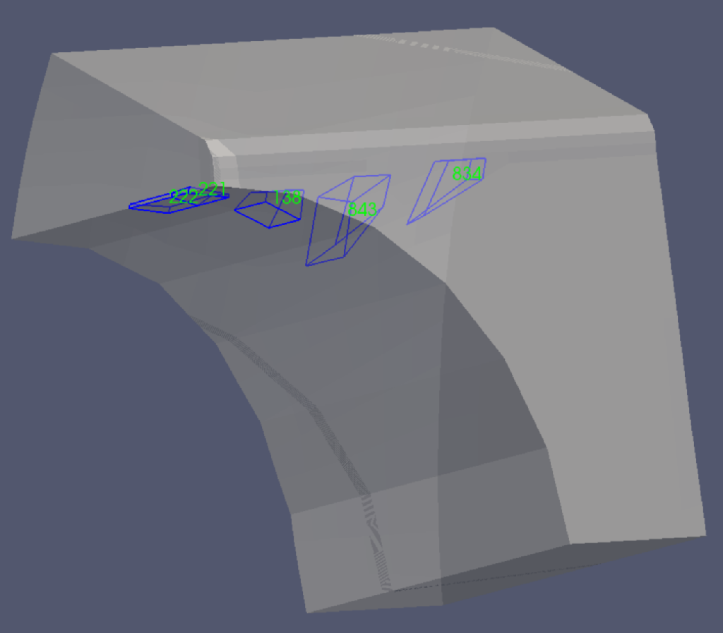
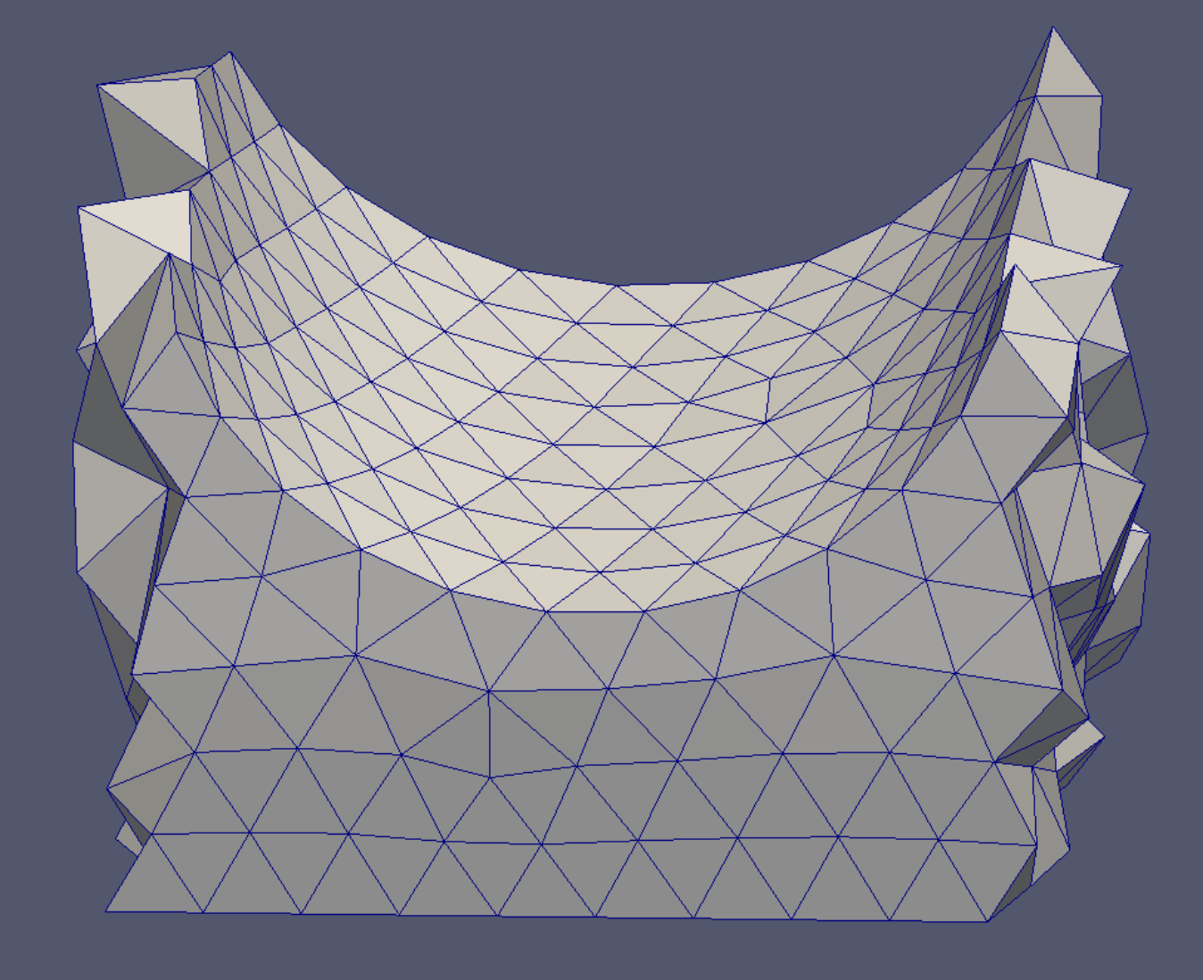
Demo 2 At right is shown the mesh for the second demo. It is a sort of semi-arch of 912 hex elements. Five of its least regular elements are illustrated, and the left three elements shown each have four surface nodes.
The top pic shows the instrument board when the file is loaded. We understand after a couple of trials that this file locks up fast, so there is no need to retain a large sample. We also discover that the Scaled Jacobian is not sensitive, and so we use a standard edge length with a small polyhedron. Then we are ready to try to improve the Diagonal. We find it resistant to change. Incidentally, it may be time to comment on the SJ Min text block in the Target panel. This value is the minimum Scaled Jacobian which is allowed to appear as the Diagonal is calculated. It is not fully dependable however, and may require some padding. Note that Diagonal calculations will not start unless the current Scaled Jacobian is equal to or greater than the current SJ Min.
Demo 3 At right is shown the mesh for the third demo. It is a quarter hole with a penetration, consisting of of 492 hex elements. Four of its least regular elements are illustrated, and none contain surface nodes. A word about Lifted’s testing algorithm may be in order. A search path is traveled twice, and in the first trip improvements are sought for nonconforming elements, and the test results stored. Scores are then sorted. At that point the initial conditions are reset, and the number of iterations are conducted which produced the highest score on the first half of the run, thus seizing the optimal value for those settings. If Lifted encounters a user-entered number in the Elem No edit box, it calculates that element and then stops. This feature is available for special effects, when the preferential sorting of the auto Execute procedure is not desired, or to skip a stuck element and do others. If the chosen element is not the worst case, then the Status message at the top of the interface must be relied on to inform the user whether or not processing the chosen element results in improvement.
The pictures at right show some panels for the third demo. The second one shows that it is easy to obtain a creditable Scaled Jacobian with this mesh. A couple of trials demonstrate a high sensitivity when calculating the Diagonal. Therefore we raise the SJ Min value to protect the Scaled Jacobian, but find it an unnecessary precaution when using the chosen settings.
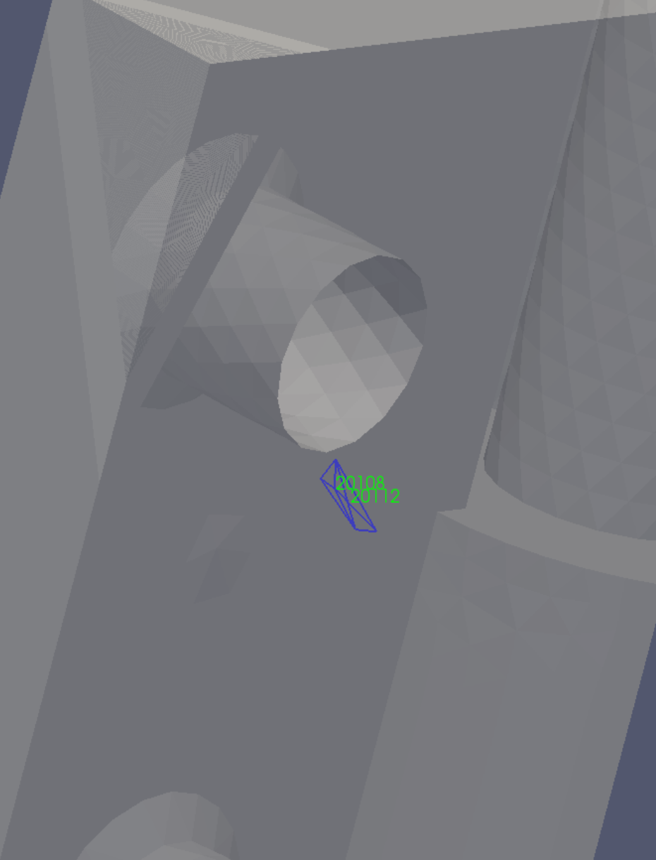
Demo 4 The pictures at right show the mesh for the fourth demo. It is a cutaway of a journal housing, consisting of 1494 tetrahedral elements. Four of the least conforming elements are shown lower right. None of them contain a surface node.
The picture at right shows the Lifted panel upon opening the mesh file. The tetrahedral analysis involves fewer edit boxes than the hex equivalent, and the unused ones are grayed out. The Verdict Edge Ratio attribute is the only one we seek, and the acceptable maximum level is judged to be 3.0. The lower pic shows the edge ratio value achieved by the settings depicted. We did not find settings which refined the results in any successive trials, although we did find a few settings which tied the outcome.
Demo 5 The mesh consists of 2967 tetrahedra. It was meshed with the Netgen subprogram within Elmer, using a default ‘h’ value. It was translated to .msh format by e2aps and then opened in Gmsh and saved as a .vtk file. (See references.) The three elements with the lowest quality rating are shown. All 9 nodes comprising these elements are surface nodes.
In view of the above situation, it is obvious that Lifted cannot alter the Edge Ratio quality level.
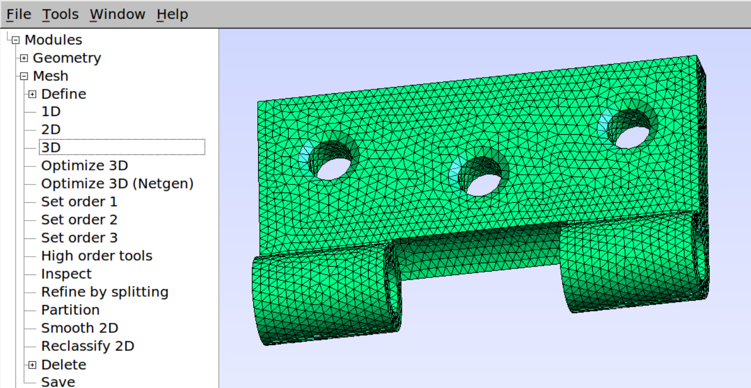
Demo 6 The next demo continues with the hinge mesh, but at a higher resolution, with ‘h’ value set at 1.0 during its construction. It consists of 41,211 elements and 7777 nodes. For the two sample defective elements shown at right, no surface nodes are present.
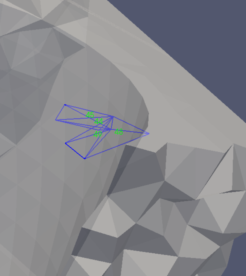
The green element labels in the Paraview view at right show the locations of the elements of interest when seen in a plan view. Lifted becomes sluggish − to the point of unusability − when working on mesh of higher density. Therefore we demonstrate how to split the mesh to speed things up. The arrow in the pic is pointing to the Paraview (version 4) icon for ‘Select Cells Through’. This drills through a mesh, capturing all included elements, resulting in the selection shown below right.
Next we use the ‘Extract Selection’ filter, obtained through the Filters menu, to break off the selection into a separate chunk, shown right.
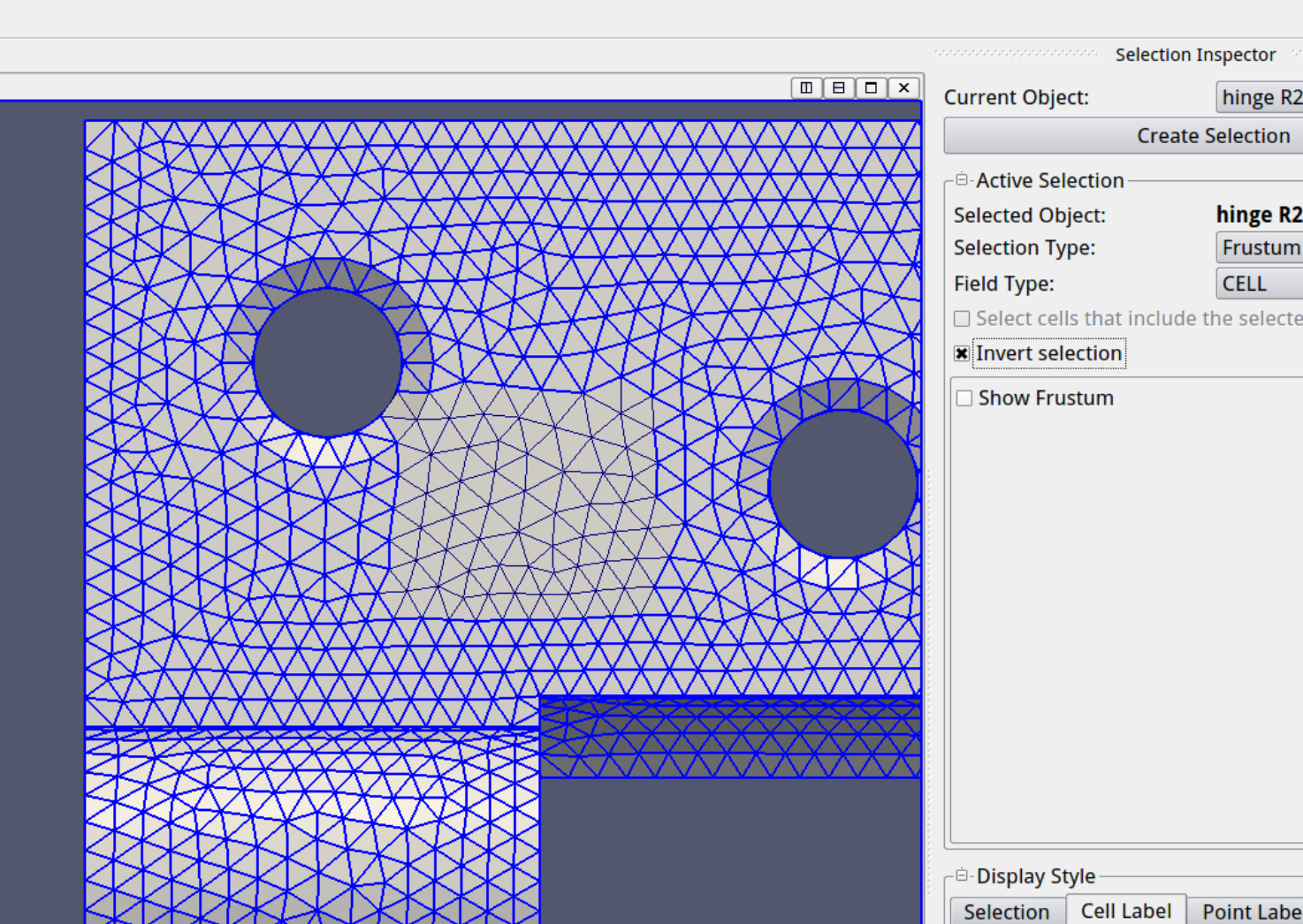
Paraview version 4 has the Selection Inspector, and from it we invert the selection, thereby capturing all the elements which were not in the original extraction. We employ the Extract Selection filter once again on the parent mesh. Now we have two pieces.
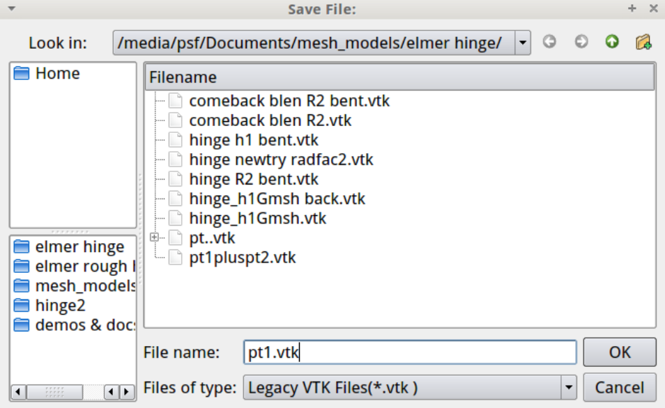
We make sure that the first chunk of elements is the only object selected or visible in the Pipeline Browser visible at the left side of the screen. Then the File⇒Save Data menu selection brings up a dialog box, in which we choose to save a Legacy .vtk file type. After saving the working chunk, we save the parent chunk in the same way.
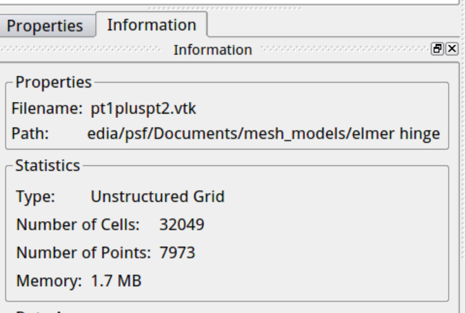
We now open the small chunk in Lifted. The Lifted operating panels for the small chunk are shown right. The settings shown produce a considerable improvement. Note that the element numbers do not correspond with the original numbering system, which referred to the pre-breakup model. Also note that because Lifted does not tamper with exterior nodes, there is no glitch or discontinuity when we put the two chunks back together.
We use the File⇒Clear option in Gmsh to clear the deck, then load the modified small chunk. We now use the option Merge under the File menu to bring in the parent chunk. The geometry matches perfectly. We press the 3D meshing button just for luck and then save as a .vtk.
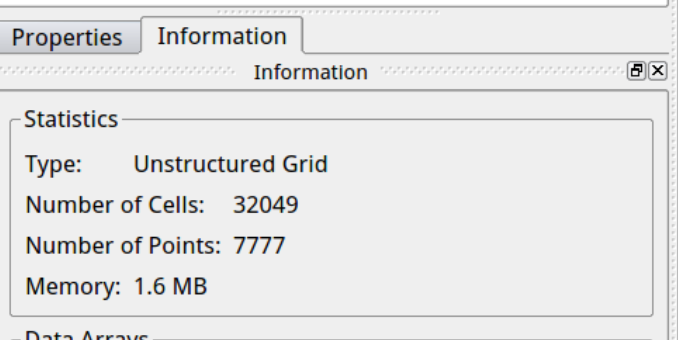
We open the composite mesh in Paraview again. Everything looks fine, but on consulting the Information tab below the Pipeline Browser we notice that the exterior nodes in the small chunk did not get merged in Gmsh with those of the parent chunk. Not a problem, we simply use the Clean to Grid filter and the duplicate nodes are absorbed, giving us the exact number of nodes we started with.
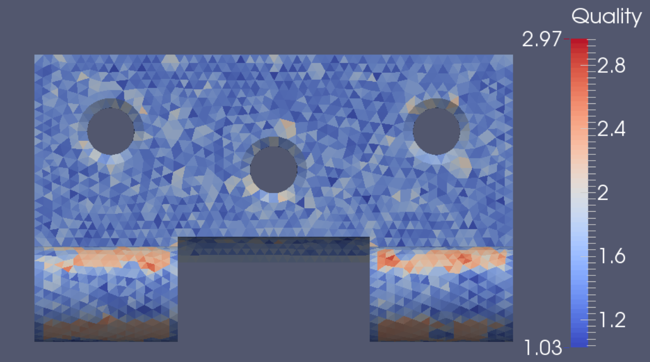
The composite mesh Edge Ratio quality shows the influence of the improved small chunk. The unimpressive score of 2.97 is due to an element or two in the parent chunk with unluckily placed surface nodes.